Global Navigation Satellite Systems Software-Defined Receivers explained. Part 2: Jamming mitigation
GNSS jamming is something I’m very familiar with and with what I’ve been involved in for most of my career. My specialist’s thesis (6-year degree, Russian alternative to bachelor and master combined) was about real-time narrowband interference mitigation for GNSS receivers with FIR-filters, I wrote several papers about that and, eventually, I became a scientific supervisor of the big antijamming and antispoofing project. In that project, I and my team have investigated various approaches for spatial (digital CRPA) and non-spatial interference and spoofing mitigation. Then we implemented them with MATLAB models and built some test benches with real hardware to test the models and algorithms with real-world data. And we’ve even designed and implemented antispoofing and CRPA antijamming receivers as working prototypes, operating in real-time! As you already guessed, this is the topic I’m very comfortable with and could talk about for hours, but I’ll try to keep it brief and concentrated.
- Part 0: Hardware and system design
- Part 1: Digital frontend
- Part 2: Jamming mitigation
- Part 3: Acquisition
- Part 4: Correlation and tracking
- Part 5: Standalone positioning
- Part 6: Advanced positioning methods
Overview and effects of the interference
Jamming is the term used for a radio-frequency interference of the GNSS signal, and it can be unintentional (like the DME landing systems for the L3/L5 subband) or harmful or intentional (jammers and other “personal privacy devices”). The goal of jamming is pretty simple: to disable the GNSS receivers in some areas. We’ll omit the reasons for this and just get to the effects and countermeasures.
The receiver, affected by jamming, will provide a deteriorated solution or even no solution at all. The presence of jamming leads to a decrease in signal-to-noise ratio (SNR) up to the point where the signal acquisition and, then, the tracking are impossible. For simplicity, we’ll assume that before the jamming mitigation the signal path is linear and the jammer signal is not distorted. For real-world applications, you’d need to look at the 1 dB compression point parameter (P1dB) of the RF frontend and the number of bits of the ADC. For example, if the narrowband tone interference is being distorted (in the frontend or by using the 2-bit ADC) it’ll turn into the multitone. It’s still possible to mitigate, but at the cost of an additional SNR.
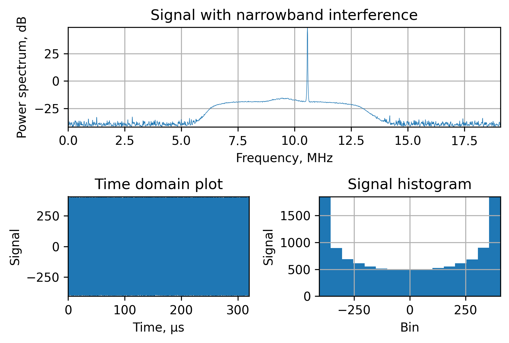
To illustrate this let’s add a tone interference to the signal we’re working on:
interference_offset = 1.023e6
interference_level = 25
signal_with_interference = np.ceil(signal_data + interference_level * np.cos(-2 * np.pi * time  * (intermediate_frequency + interference_offset)))

PlotSignal(signal_with_interference.astype(np.int8), fs, 'Signal with narrowband interference')
In the following figure, we can see the main interference tone and some harmonics due to the quantization error (ceil + cast to int8 for the following clipping demonstration). Another interesting point here is in the histogram. Usually, in the lack of interference, the signal histogram is bell-shaped due to the normal distribution of the input signal, which is caused by the satellite signal being buried ~20 dB beneath the noise. However, if we add the narrowband interference, it’ll shift to the ramp shape, since the harmonic signals “spend” most of their time in their upper and lowest values.
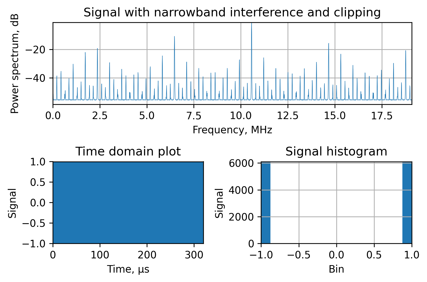
When the GNSS receiver uses low-bit ADCs, they’re clipping the input signal. For example, let’s demonstrate the simplest case of the 1-bit ADC, which is effectively a comparator. When you clip the sine into two levels it becomes a square wave. As you may know, the spectrum of the square wave is full of harmonics with a $\frac{sin(f)}{f}$ envelope. This is exactly what we see in the figure below:
Narrowband interference
The narrowband (single-tone and multitone) interference is a common thing to spot in the GNSS receivers. Since the signals are weak, it’s easy to pick up some spurs from both external and internal equipment. There are two approaches to interference mitigation, based on the domain the filtering is performed: temporal and frequency. The former is more suitable for hardware-oriented approaches or systems with very limited resources, while the latter is more software-friendly and provides better results.
Digital filters approach
There are two kinds of digital filters: finite and infinite impulse response (FIR and IIR correspondingly). The main difference between them is the latter being recursive with the possibility of being unstable. Another downside to the IIR-filters is that there’s no way to design a filter with a linear phase. However, there’s a significant advantage: it’s possible to design the IIR-filter with the same attenuation characteristics of a significant less order, therefore, less silicon area.
For GNSS jamming mitigation it’s reasonable to go with the FIR-filters because it’s possible to design a filter with a linear phase response. During my research, I’ve found a very elegant and computationally-efficient design method I’d like to share: the frequency response sampling method. To demonstrate this algorithm I’ll use two additional tones at -1.023 MHz and 2.046 MHz on top of the translated signal:
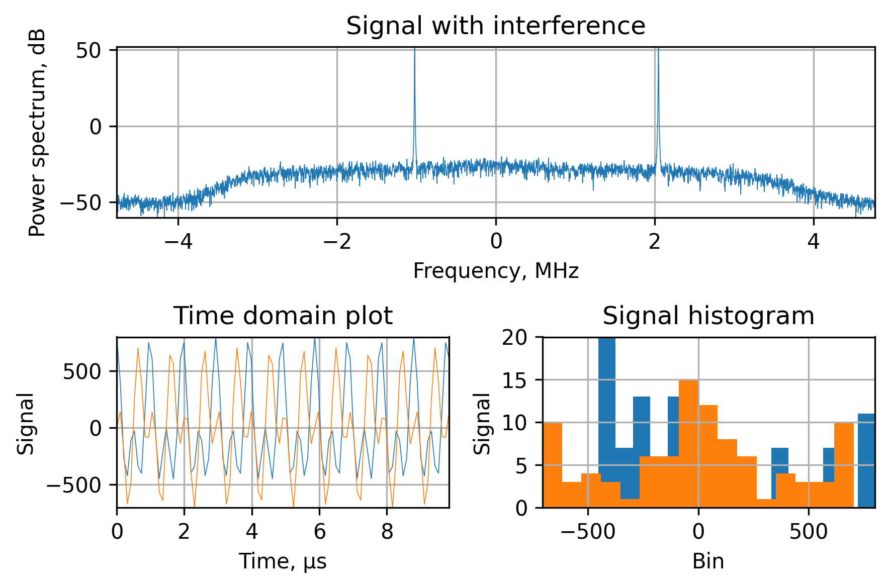
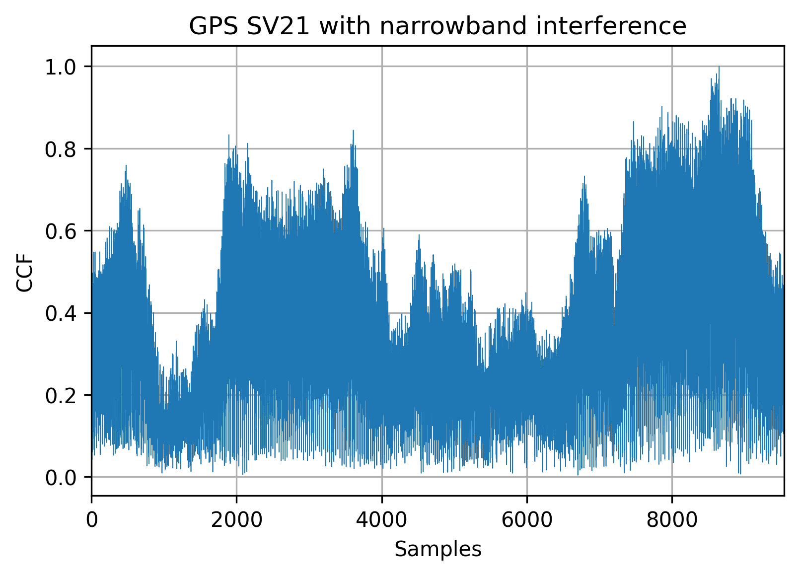
If we use such a signal as-is with the matched filter we won’t be able to distinguish the signal from the noise:
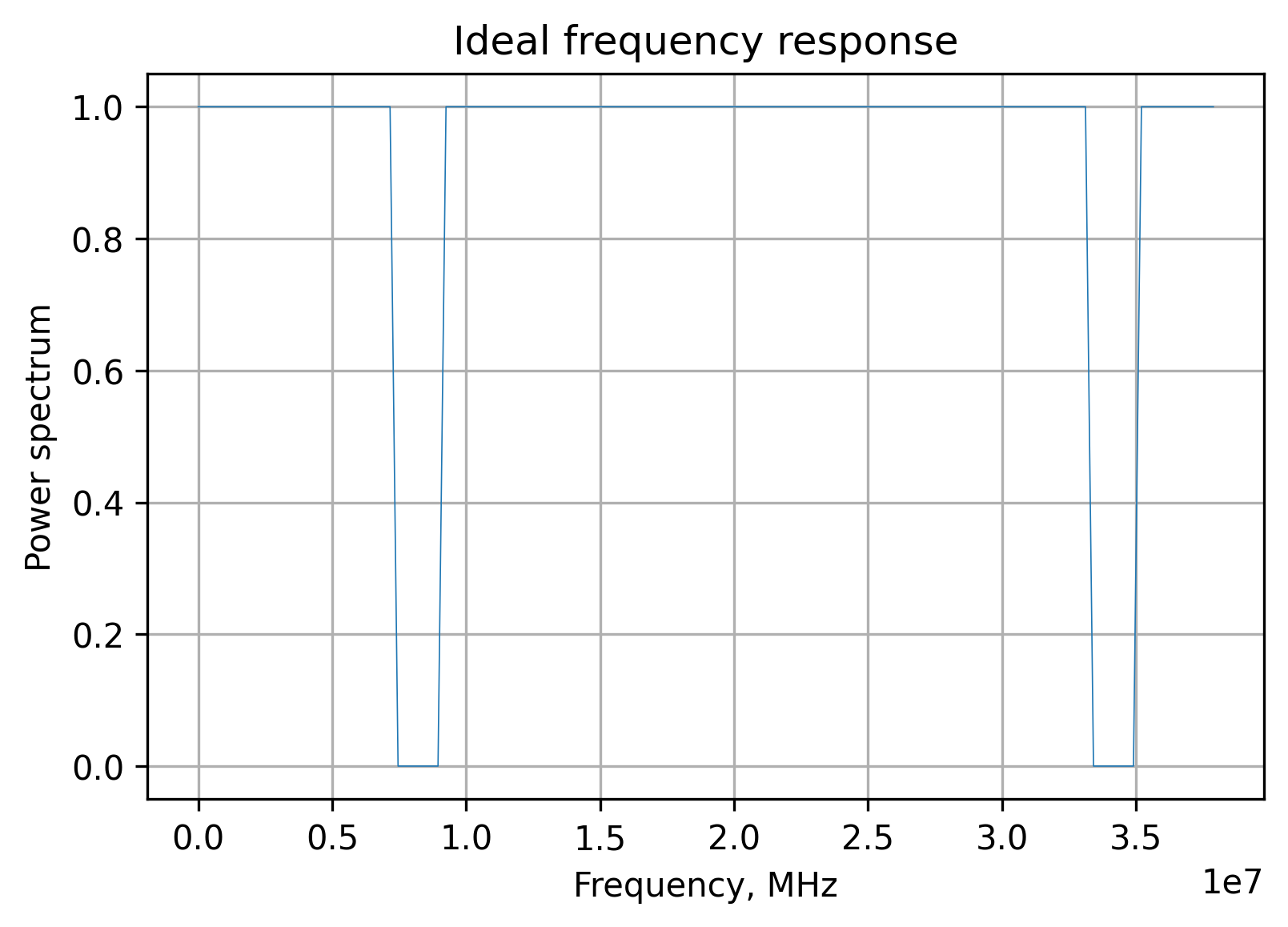
The idea and the algorithm are simple: create an ideal frequency response with zeros for frequencies to suppress and ones otherwise:
The second step is to apply the phase multiplier to create a linear phase response. The preliminary impulse response is obtained by the inverse Fourier transform, but such a system is susceptible to the Gibbs phenomenon, resulting in a massive suppression performance degradation. As a final step, to mitigate this effect, a window function is applied.
All those steps are implemented in the GetIr function, which is in the composed Jupyther Notebook. The resulting impulse response with a linear phase and nulls at the frequency locations of the interference looks like this:
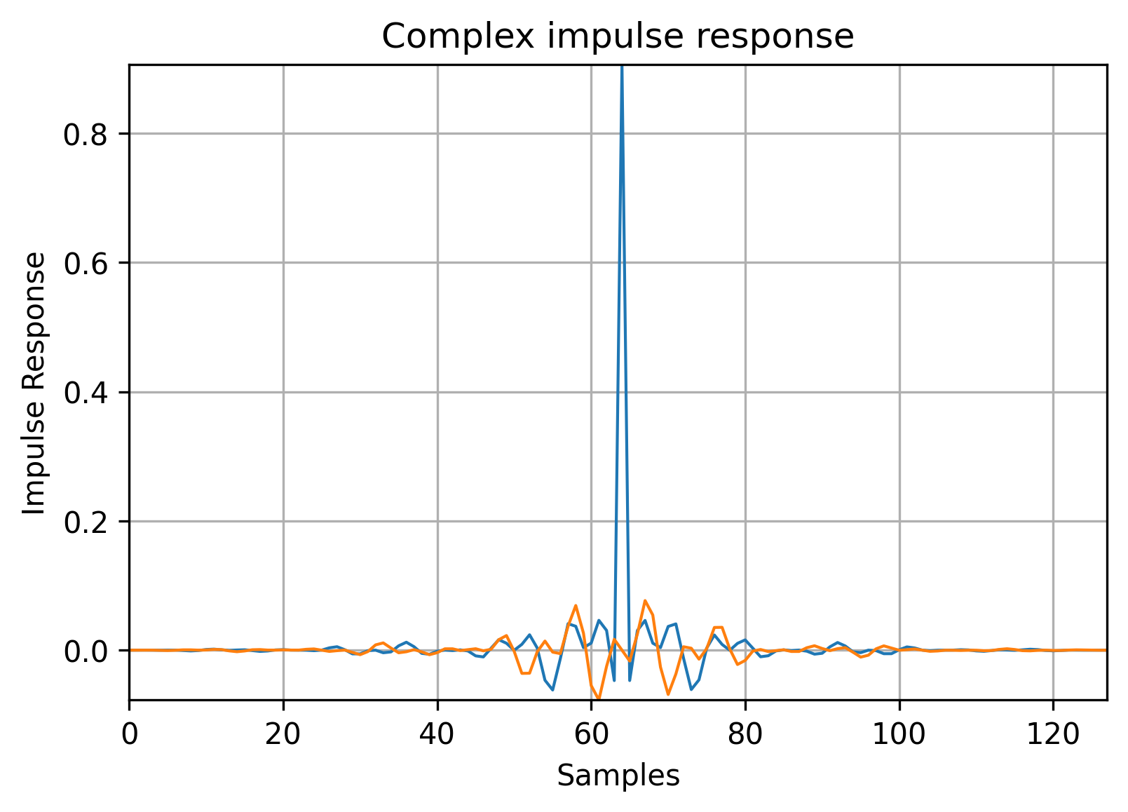
Bear in mind, that since the input signal (and interference) is complex, we’d need a complex frequency response to mitigate it and, therefore, a complex impulse response. After the complex FIR processing, we can observe the mitigated interference:
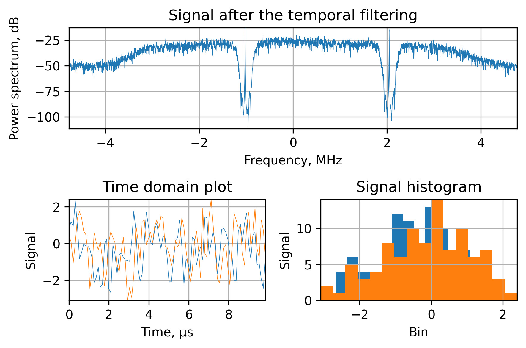
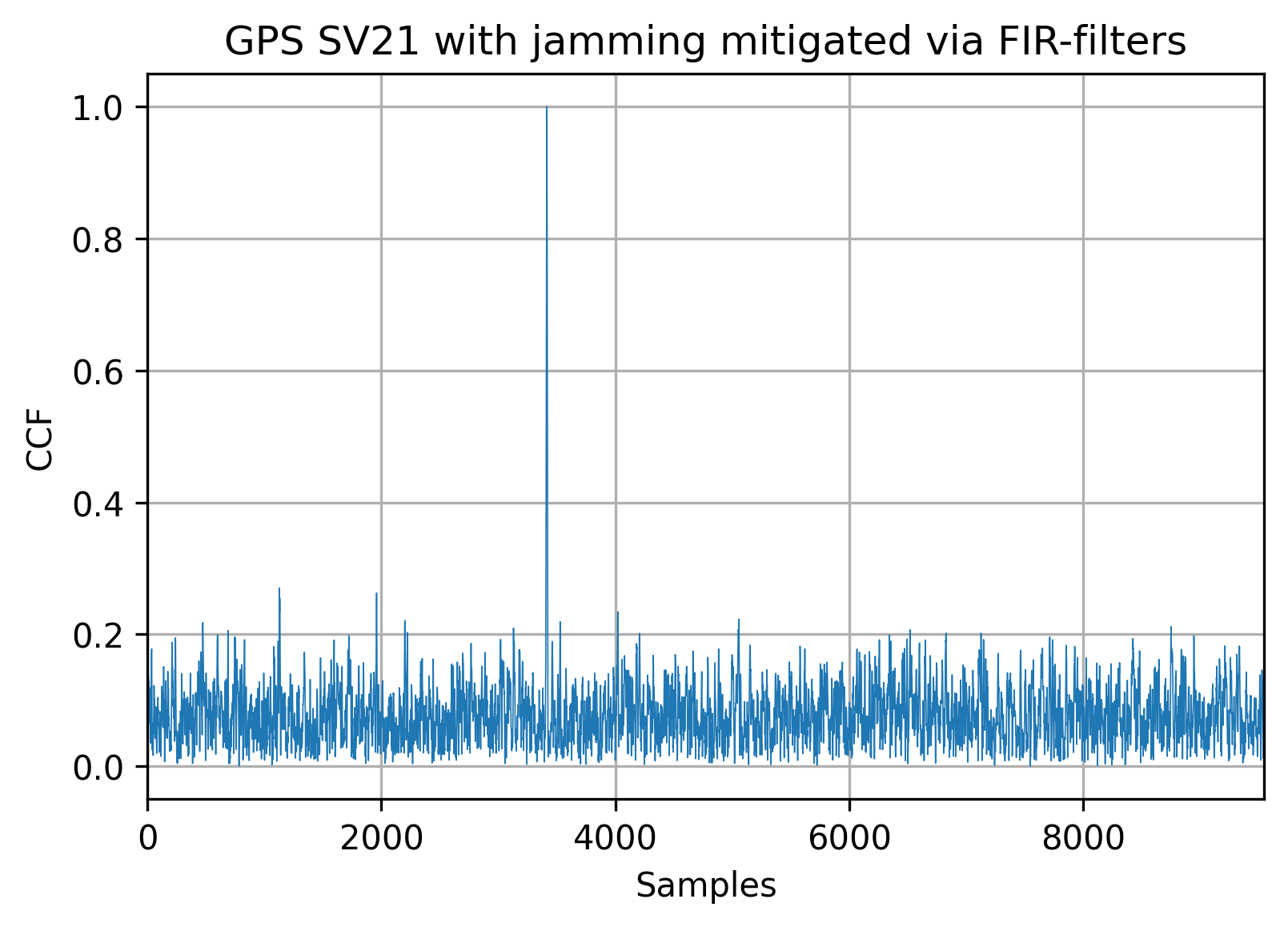
The temporal processing will allow to suppress the narrowband interference and locate the satellite signals:
Frequency domain approach
The frequency-domain approach is more demanding in terms of memory but provides much better results. The main idea behind it is to detect the interference, zero out the corresponding frequency components of the input signals Fourier transform and then perform an inverse transform to get a signal for the following signal processing.
Another benefit of frequency-based processing is the lack of filter-induced group delay. This is just a constant for a traditional linear-phase FIR-filter, but it’s another thing to keep in mind and pass to the observable block and, therefore, a potential source of errors.
For the same signal and interference mix we’ve used in the temporal approach demonstration, we may observe the superiority of the frequency domain-based approach:
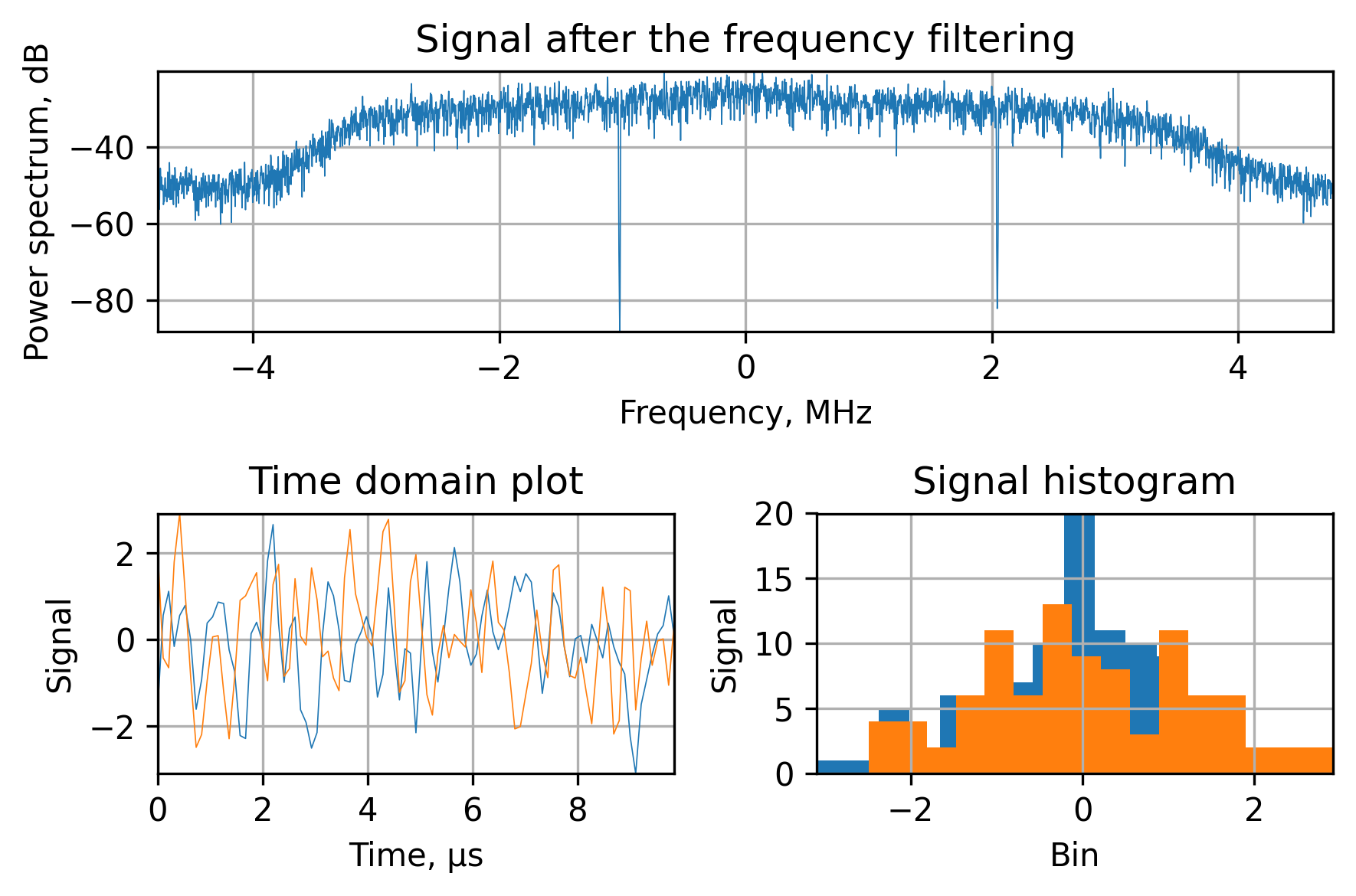
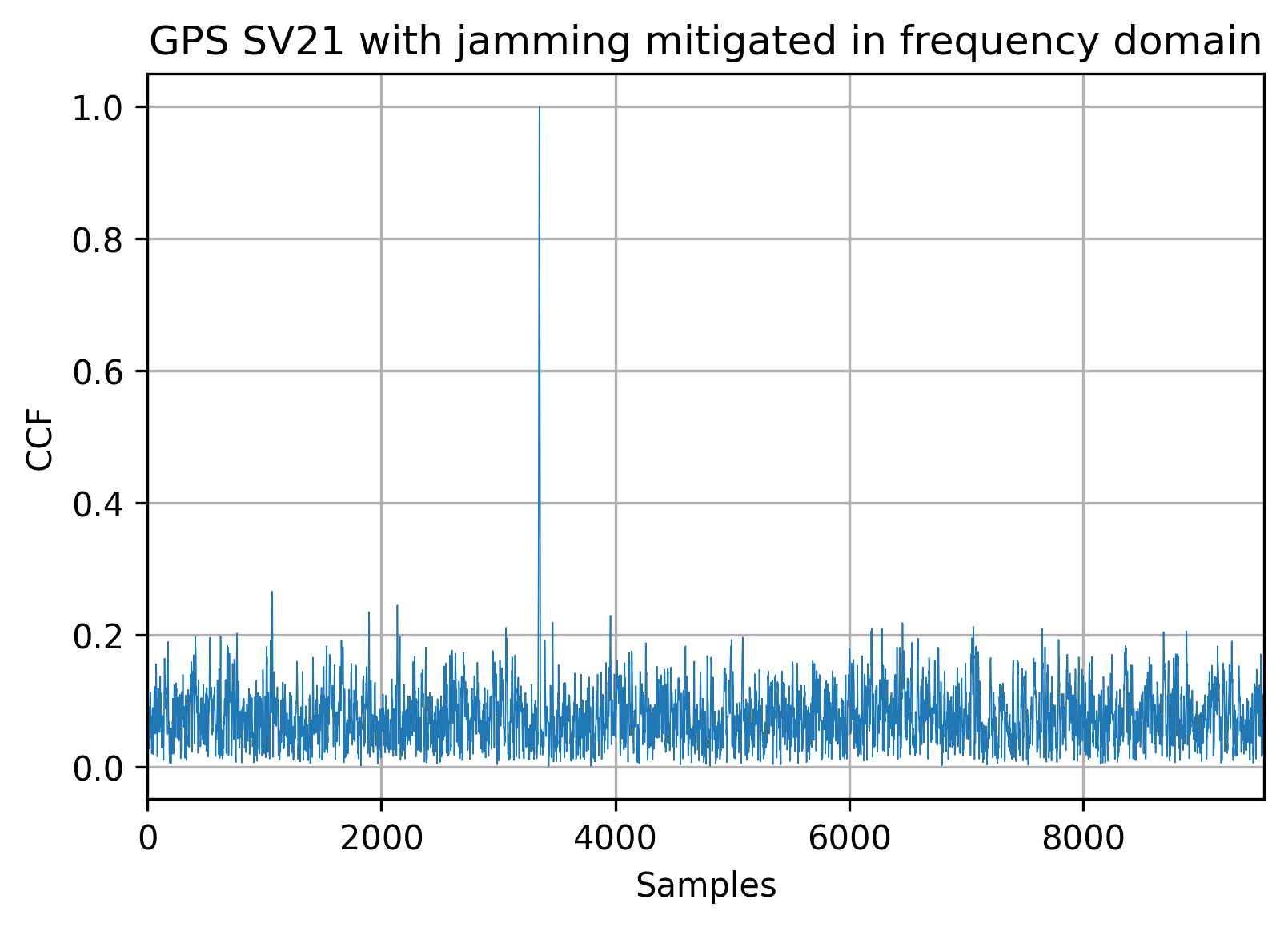
The matched filter will again prove that we’re suppressing the interference well and the signal can be found:
Wideband interference
Unlike the narrowband interference, the wideband is covering the whole frequency band of the GNSS signals. One of the most common and easy-to-assemble devices produces a chirp signal. A chirp or sweep signal is a kind of signal in which the frequency is varying over time. The most common is the linear frequency sweep interference, but there’s an interesting ‘tick’ swept frequency signal worth investigating (more information in Impact Analysis of Standardized GNSS Receiver Testing against Real-World Interferences Detected at Live Monitoring Sites by NSL). There are also some debates going on in academia regarding the pseudo-white noise interference, but I’ve never seen it implemented in the real world due to the heavy practical limitations like the crest factor.
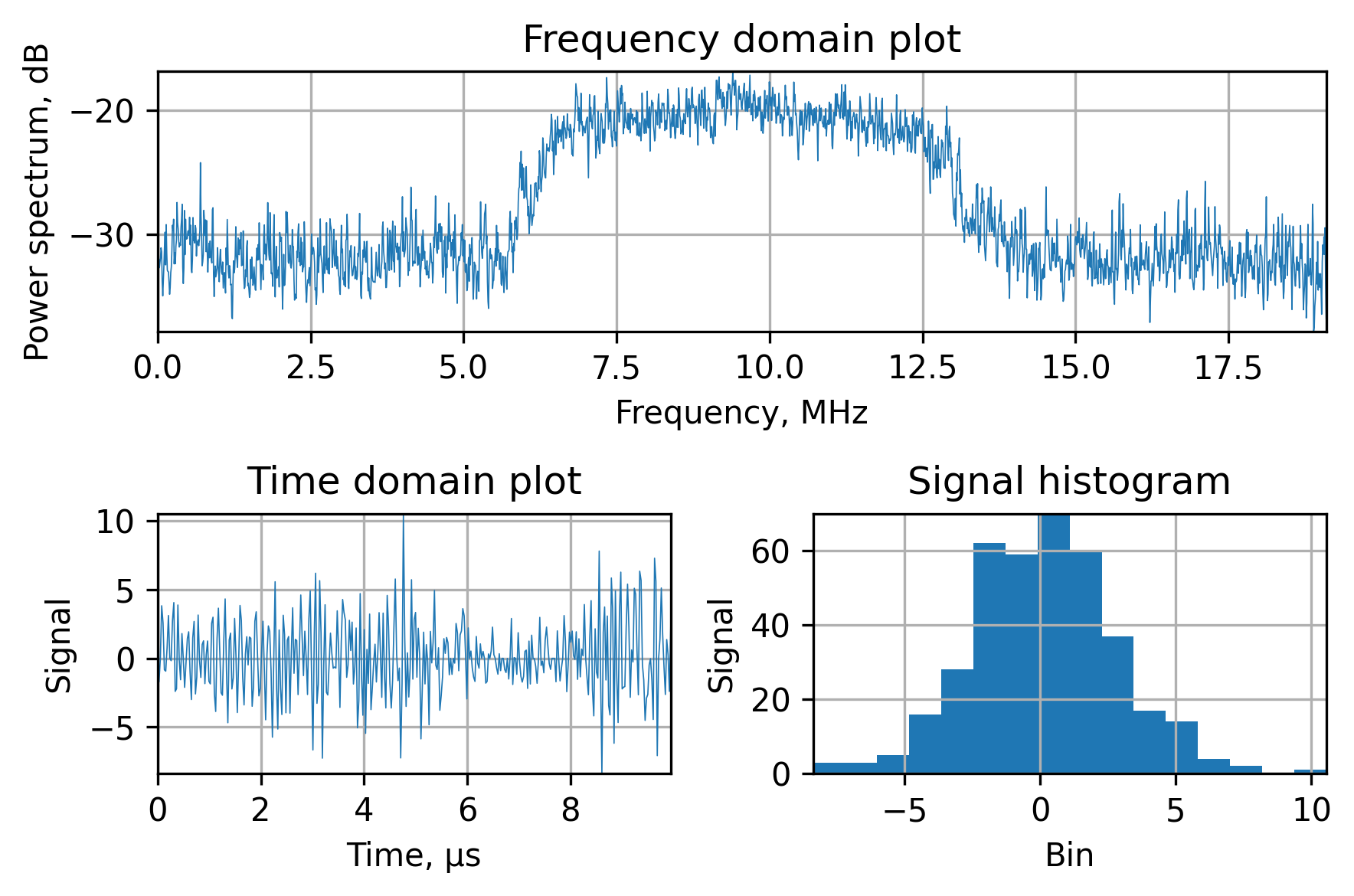
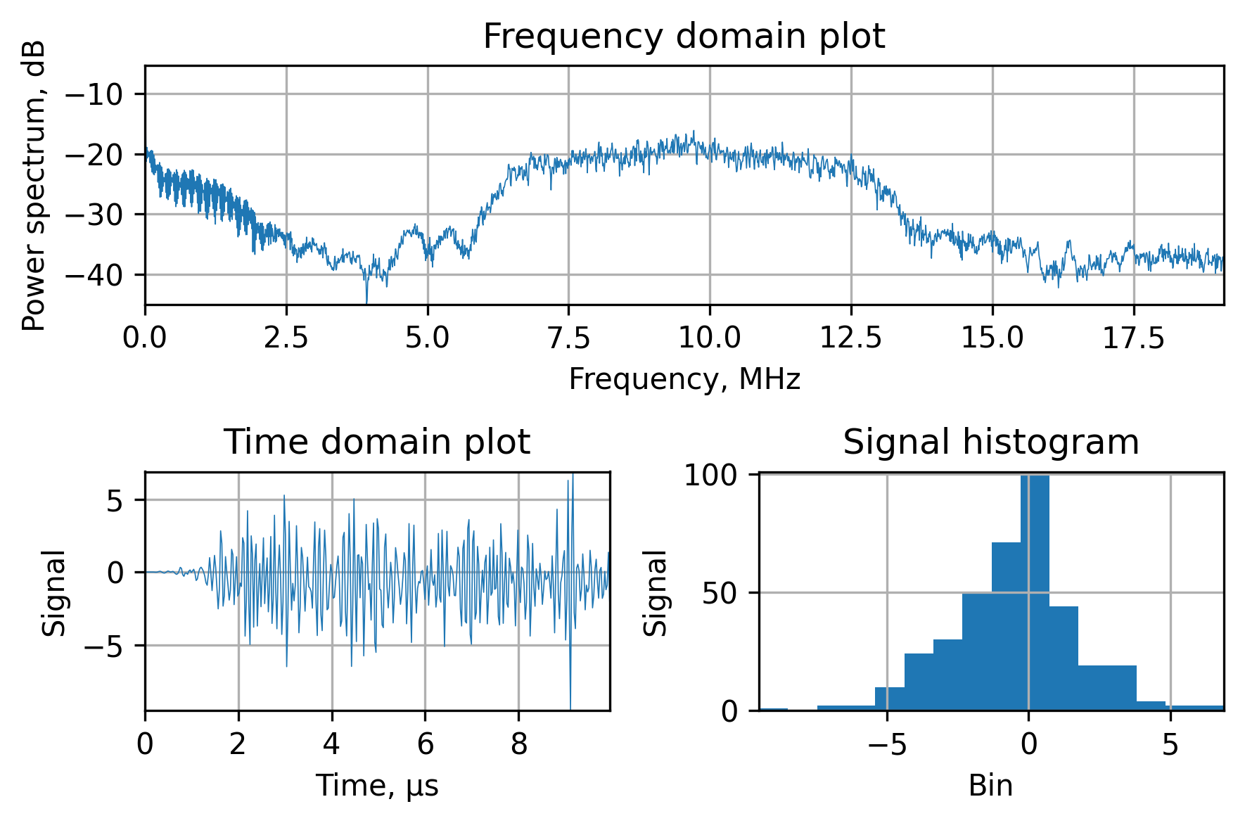
Usually, wideband jammer signals would look like this with an additional (not displayed here) shape of the RF filter in the antenna:
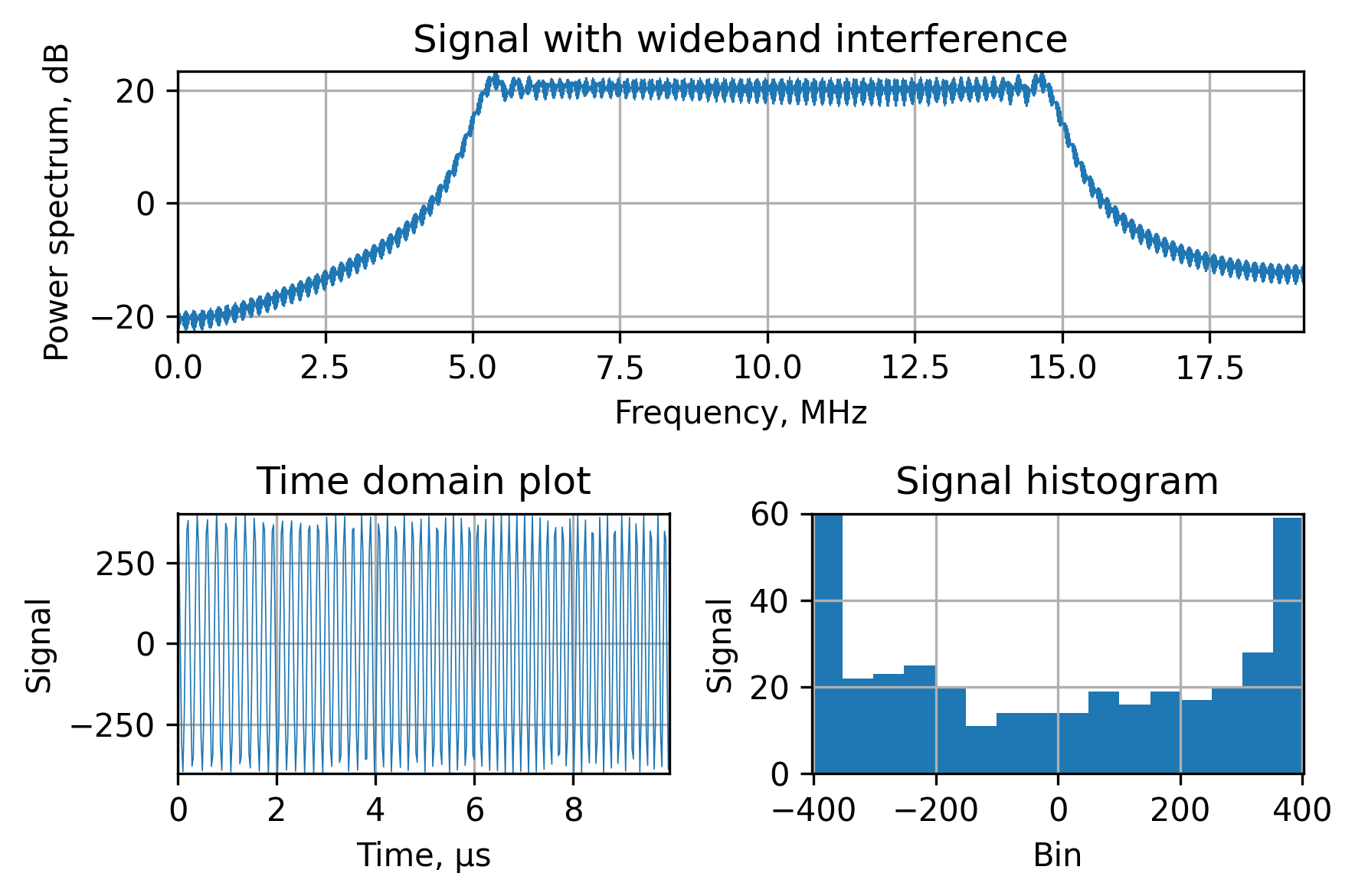
As you can see in the figure above, a regular Fourier transform will render all the efforts useless, since it’s impossible to separate the jammer signal from the satellite signal.
To get around this limitation we can use an algorithm called Short-Time Fourier Transform (STFT) and plot a time-frequency spectrum dependency called a periodogram. It splits the input signal into overlapping segments and calculates the Fourier transform for each of them independently. The length of the segments is selected to match the time resolution, or, simply put, the portion of the signal where the frequency of the interference is relatively constant.
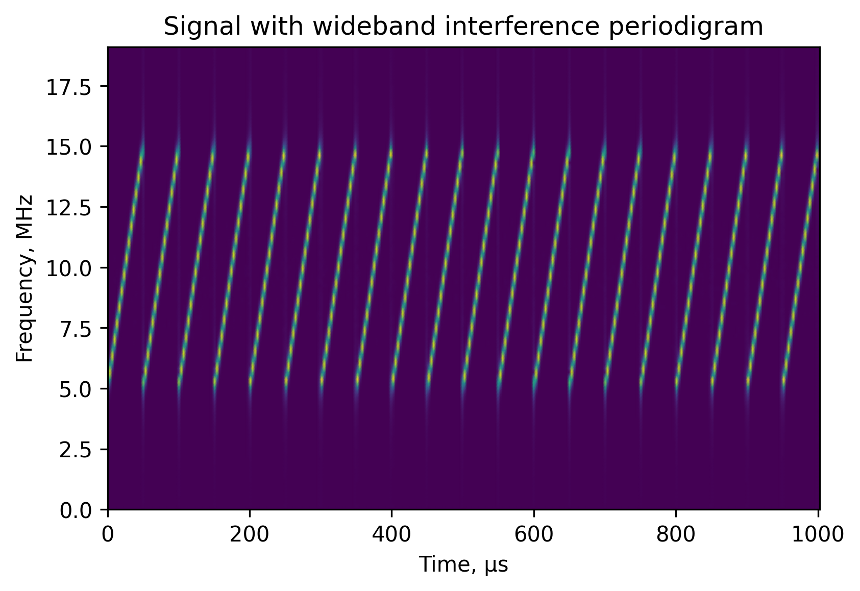
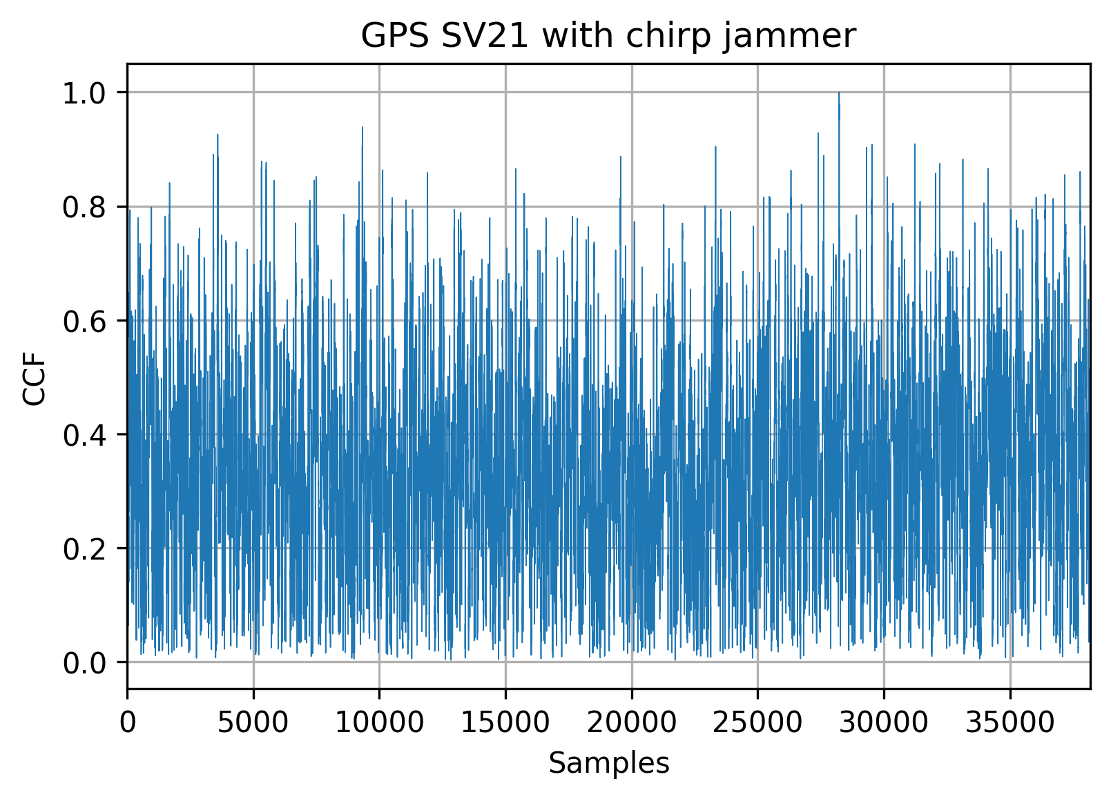
This kind of jammer is very efficient, as you can see in the matched filter output:
Digital filters approach
The approach I’ve tested numerous times is described in the Chirp Mitigation for Wideband GNSS Signals with Filter Bank Pulse Blanking paper. It splits the input signal into the $N$ non-overlapping subbands with digital filters followed by the blanking device. The blanker compares the magnitude of the filtered signal with some threshold and, if it’s exceeding the threshold, zeros the signal. Afterwards, the subbands are summed to reconstruct the whole signal.
For example, to synthesize the filter bank for this approach we can use the following Python code. This is by no means optimal and should be reviewed and investigated much further for the production-grade receiver, but it works for demonstration purposes.
bandwidth = 0.5e6
frequency_start = 7.5e6
frequency_stop = 11.5e6

frequency_bands = []
current_start = frequency_start
while current_start < frequency_stop:
  frequency_bands.append([current_start, current_start + bandwidth])
  current_start += bandwidth

filter_bank = []
for current_range in frequency_bands:
  filter_bank.append(signal.firwin(512, current_range, width=None, window='hamming', pass_zero='bandpass', scale=True, nyq=None, fs=fs))
This code will generate the filters with the following frequency responses:
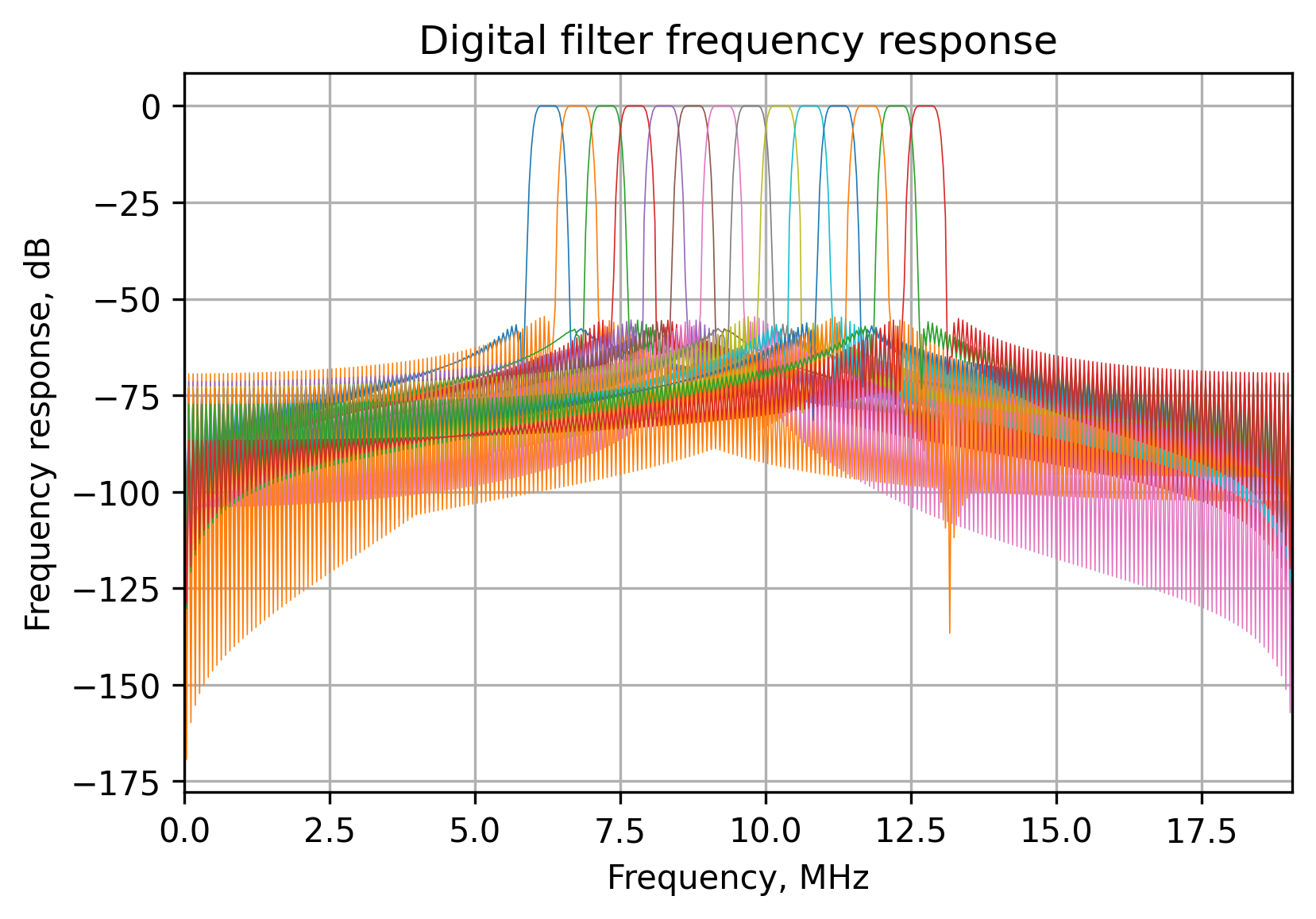
Modern chirp jammers have a sweep period of around 20 to 100μs and the described method effectively blanks each subband multiple times during each accumulation period.
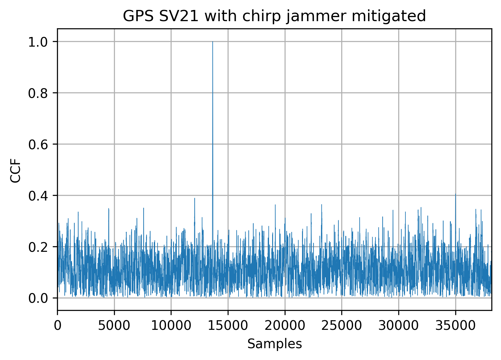
Using this approach we can achieve this kind of mitigation:
Even though the cleared spectrum doesn’t look very similar to the input one (before jamming), the satellite signal beneath the noise floor is still there, and can be acquired and tracked:
Frequency domain approach
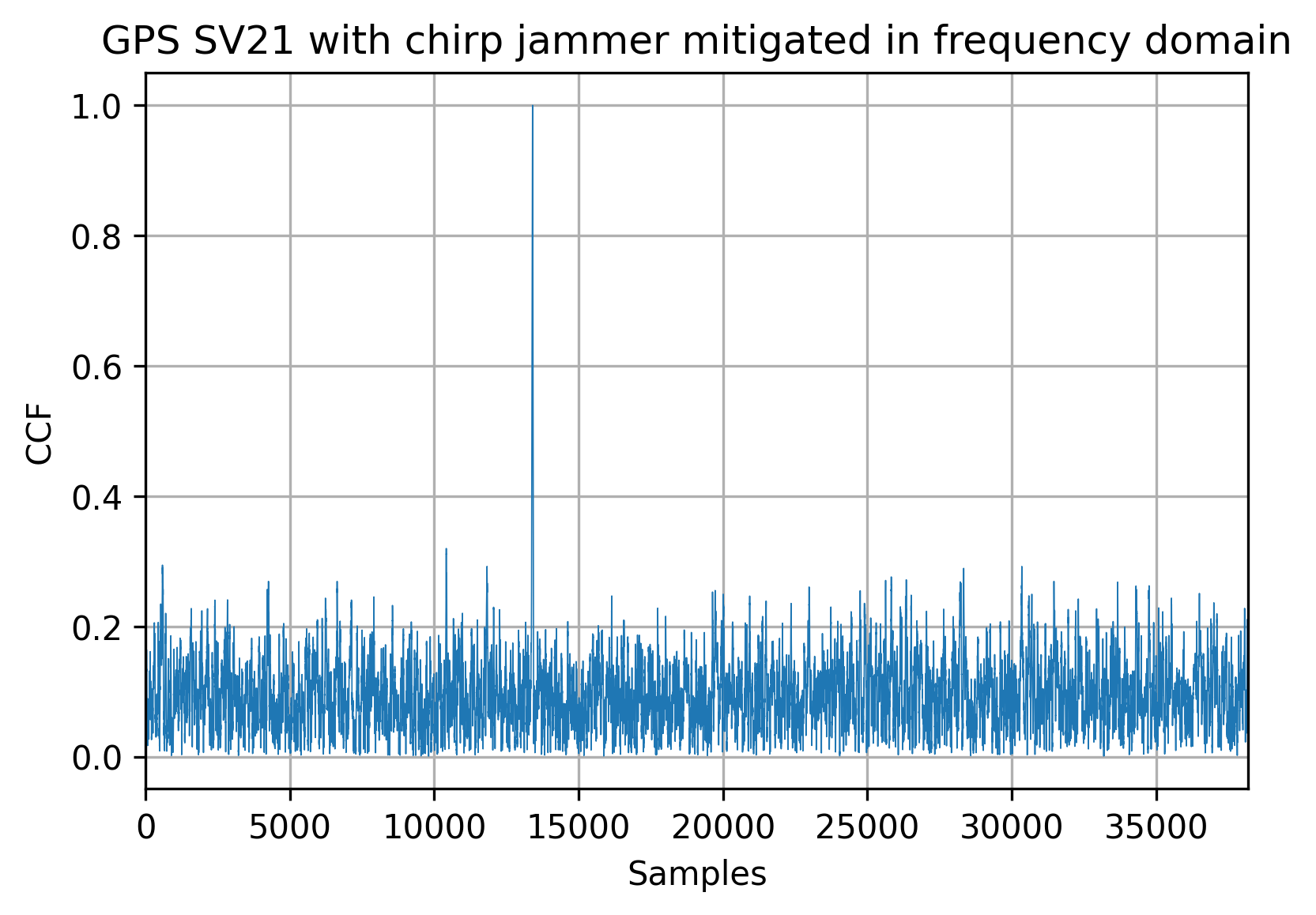
As I’ve mentioned earlier, it’s nearly impossible to distinguish between the jammer and satellite signals with the regular Fourier transform, which is why we’re using the STFT for the signals with wideband interference. The segments of the STFT are divided in a manner to keep the jammer frequency relatively constant. With that in mind, the interference is mitigated the same way as in the narrowband case.
Like the temporal pulse blanking approach, the signal is detectable after the jamming mitigation:
Space-based approaches
The most advanced jamming mitigation algorithms use space-time processing via the special antennas called antenna arrays. It is possible to manipulate levels and phases from each individual antenna element to modify the equivalent antenna radiation shape to form nulls and focused beams in the combined signal.
Unfortunately, since this approach requires multiple antennas and multiple synchronized RF frontends, it drastically increases the device cost and is rarely used for the traditional (civil) GNSS receivers.
The main idea behind the space-time GNSS processing is to fix the signal from the reference antenna element and to manipulate the levels and phases of the other elements to minimize the output power. Since the GNSS signal is well below the noise floor, everything exceeding it is considered to be an interference and should be mitigated.
Since there are much fewer openly available datasets from antenna arrays, I’ll leave this chapter without examples, possibly to return and revise in the future.
A note about spoofing
It is a quite controversial topic whether to treat spoofing as interference or not. In my personal opinion, since the spoofing detection and mitigation approaches are vastly different from the antijamming algorithms, they should be discussed separately.
There are two ways to counter the spoofing threat:
- Antenna-based via space-time or space-polarization processing. The latter may require a special antenna and is being investigated by Septentrio.
- Individual satellite signal processing with multi-decision acquisition parallel tracking and decoding. With that approach, the receiver will track all the copies of the signal simultaneously followed by duplicate rejection and grouping or clustering. After that, the cluster with the higher confidence is selected as a PVT candidate.
This is a deep and interesting topic like spatial processing, I intend to get back to it in the future.
Summary
GNSS signal jamming is a major threat in the current world. Thankfully, some algorithms and countermeasures allow for preserving the resilient PNT even in case of major interference.
We’ve inspected temporal and frequency-based approaches to mitigate narrowband and wideband interference, well suited for both traditional and software-defined receivers.