Global Navigation Satellite Systems Software-Defined Receivers explained. Part 1: Digital frontend

- Part 0: Hardware and system design
- Part 1: Digital frontend
- Part 2: Jamming mitigation
- Part 3: Acquisition
- Part 4: Correlation and tracking
- Part 5: Standalone positioning
- Part 6: Advanced positioning methods
Overview
In software-defined and software-oriented GNSS receivers, systems engineers can decouple the satellite signal processing into two separate stages: group and individual.
- Group signal processing is performed on the whole subband of the signal spectrum without distinguishing the signals of the individual satellite vehicles (SV). This is implemented by the digital frontend block, where the number of channels is roughly the number of processed signals (GPS L1 C/A, GLONASS L1OF etc.).
- Individual signal processing is the traditional digital channel explained in-depth by many authors [Kaplan, Springer]. This will be explained in the Part 4: Correlation article.
The digital frontend may be perceived as a signal conditioner, the purpose of it is to prepare the input signal for the subsequent processing: translate the signal spectrum, reduce the data rate, remove interference and pack the signal in a format, suitable for the correlator.
There are two major beneficial aspects of using the digital frontend:
- As I’ve mentioned earlier (Frequency plan), ADCs usually operate on a fixed sampling rate, which often is not optimal for the specific signals. The resampling part of the digital frontend allows us to reduce the sampling rate individually for every group signal, hence reducing the computational load on the correlators.
For example, if the ADC is providing samples with 79.5 MHz and we want to develop a narrowband GPS L1 C/A timing receiver we can downsample the incoming signal by the factor of 20 (down to 3.975 MHz). In that case, we’ll perform one spectrum translation on the high frequency and resampling, but the following N (by the number of satellites) translations and correlations would take 20 times fewer operations for both mixer and correlator.
- By separating the group and individual SV processing it is possible to separate the timing approach as well. For real-time receivers (implemented with FPGAs or ASICs), the group processing is often implemented synchronously with the ADC clock (~ tens of MHz), but the resulting signal can be saved to the internal memory and then processed in a co-processor manner, running as fast as it can be synthesized/clocked in case of FPGA or ASIC accordingly. The benefit here is that the same hardware can be reused for the benefit of silicon area optimization.
The second aspect is not so relevant for the PC-based receivers, since it’s virtually impossible to organize the sample-based streamed data, and those kinds of receivers are asynchronous by design.
Mixer
Mixers are the devices used to translate the signal, which results in the shift in the frequency domain. Most digital mixers are complex and perform the multiplication of the input signal with the complex exponent: \[result(t) = input(t) * e^{-j(2\pi ft + \varphi)}\]
With the transition to the digital signal processing and samples, this can be re-written as: \[result[i] = input[i] * e^{-j(2\pi i\frac{f}{f_s} + \varphi)}\]
For the demonstration, I’ve used a simple Jupyter Notebook so you can try it yourself.
First of all, we download and read the data buffer. For the sake of simplicity of the demonstration I’ll convert the data to the floating-point:
file_link = 'https://www.dropbox.com/s/b2il4hnu30fup7c/GPSdata-DiscreteComponents-fs38_192-if9_55_partial.bin?dl=1'
filename = 'GPSdata-DiscreteComponents-fs38_192-if9_55.bin'
fs = 38.192e6
intermediate_frequency = 9.55e6
request.urlretrieve(file_link, filename);

signal_data = np.fromfile(filename, dtype=np.int8).astype('float')
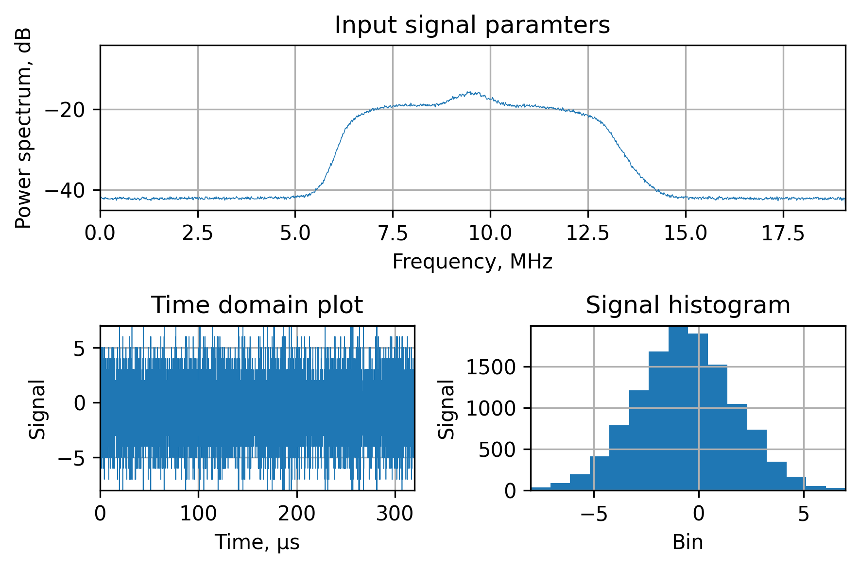
To illustrate the data properties, we’ll plot the power spectrum via Welch’s method, the first 100 microseconds and the signal histogram:
As it was mentioned earlier, to translate the signal we’d have to multiply it by the complex sine:
time = np.arange(signal_data.shape[0]) / fs
sine = np.exp(-1j * 2 * np.pi * time  * intermediate_frequency)
translated_signal = signal_data * sine
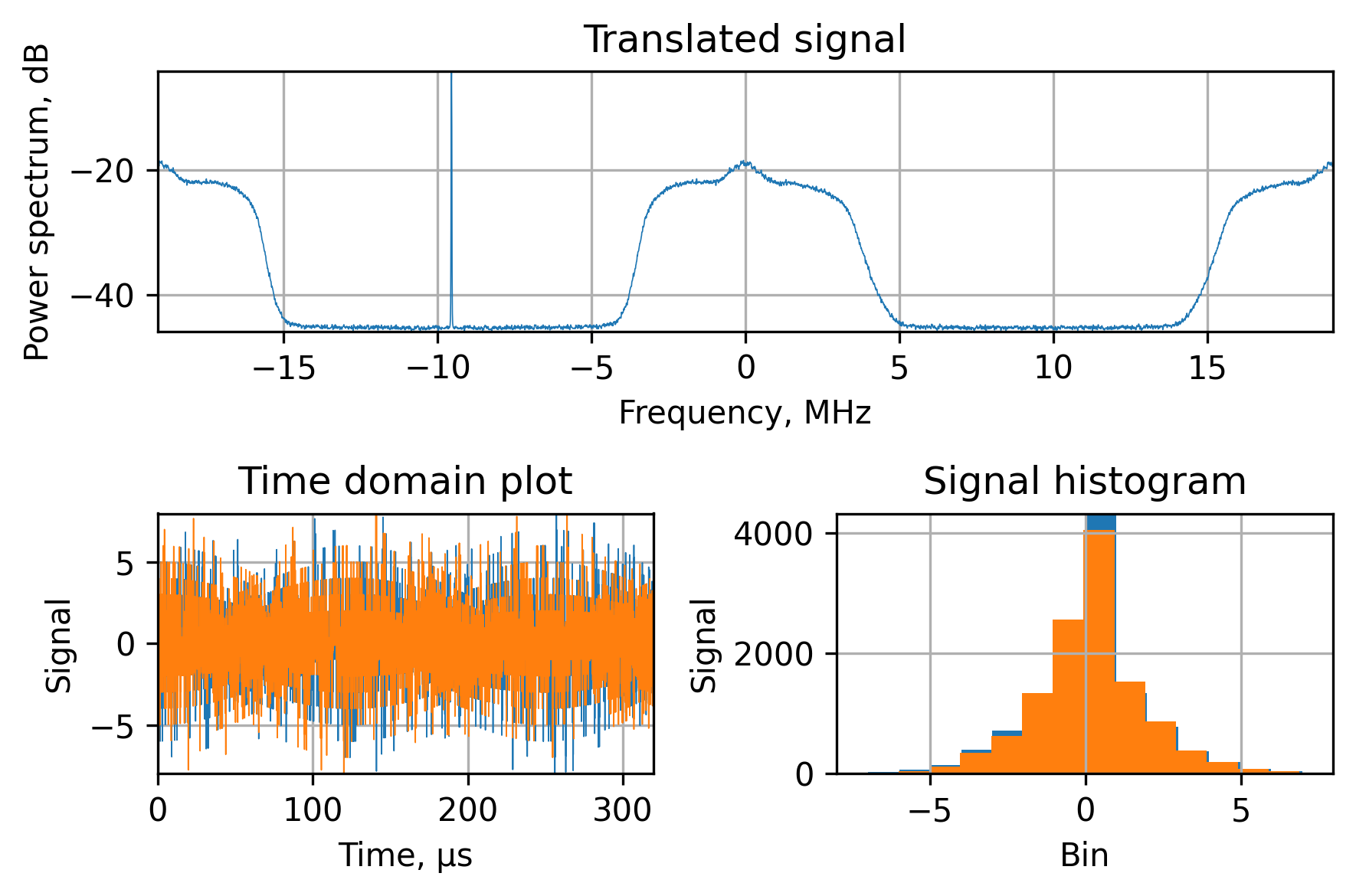
Here are the key points that can be observed in the results of the multiplication:
- Since we’re multiplying the real signal with the complex exponent we can observe the spectrum repetition in the frequency domain plot. This is present because the real signal has a spectrum that’s symmetrical relative to the $\frac{f_s}{2}$. This won’t affect the following processing as long as we have a proper anti-aliasing filter in the downsampling block.
- The peak at -9.55MHz is the DC part of the spectrum being translated to the negative intermediate frequency.
- The multiplication operation is linear and doesn’t change the nature of the underlying signal.
Verification of operations
It’s always good to check and test your algorithms and operations throughout the development process. In those articles, I’ll omit most of the tests for demonstration purposes but I intend to keep the most visual and high-level test: the matched filter test.
The matched filter is an optimal filter, designed to maximize the signal-to-noise ratio. It has a complex frequency response conjugated to the complex frequency response of the signal it is designed to detect. According to the convolution theorem, we can substitute the circular convolution with the multiplication in the frequency domain. Therefore, the Python code for the matched filter is straightforward:
def MatchedFilter(signal_data, code_data):
  return np.fft.ifft(np.fft.fft(signal_data) * np.conj(np.fft.fft(code_data)))
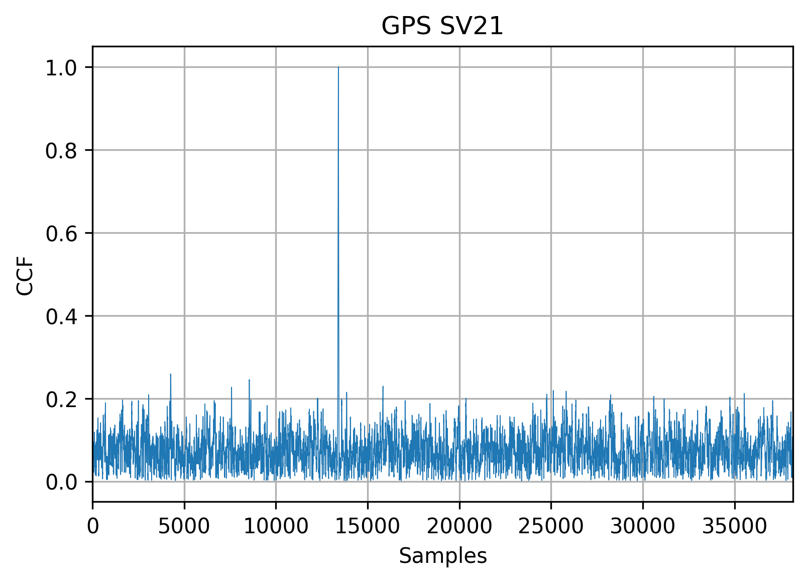
Since we’re working on a well-known GNSS dataset, we can use external information about the signals present. I’ll use a GPS SV21, but any satellite can be used. With known Doppler offset this test performs an additional spectrum translation, upsamples the PRN code and calculates the matched filter output, which is then being normalized and plotted:
Hardware-friendly optimizations
It is worth pointing out that digital signal processing devices and GNSS receivers in particular rarely operate with floating-point values and usually work with integers.
:information_source: Interestingly, with my research on PC-based software-defined receivers,
fp32digital signal processing routines significantly outperformed the integer-based ones, while both approaches were implemented with the Intel® Integrated Performance Primitives library. I’m looking forward to evaluating the performance and accuracy of the lower-resolution floating-point values (likefp16,bfloat16or evenfp8) but without the optimized libraries and hardware support, this kind of research isn’t available yet.
The most hardware-friendly approach for the integer-sine is a numerically controlled oscillator (NCO) with the corresponding phase-to-value sine table.
NCO may be viewed as an arbitrary precision unsigned integer with the full-scale treated as a period of the target function. NCOs have two main input parameters: phase accumulator value (phase) and an adder (relative frequency). The bit depth of the NCO is directly related to the possible frequency precision it’s able to achieve. NCOs are widely used in various digital signal processing systems for both receivers and transceivers.
To create a sine with an NCO it’s required to precalculate the lookup table that will convert the NCO phase into the amplitude of the target function. Usually, the number of these lookup table entries is much smaller than the resolution of the NCO. To address this issue and keep the frequency resolution of the NCO the index in the lookup table can be achieved as the higher $M$ bits of the $N$-bit phase accumulator.
Another thing worth pointing out: if your lookup table is filled with integers (scaled sine values) you may find that the bus width is not enough for several consecutive operations. For that matter, you might use a so-called normalizer block, which is a scale-down operation. To illustrate this: your input is an 8-bit and the lookup table is also using 8 bits to represent the sine. When you multiply the two numbers the worst-case scenario is that you’ll require 17 bits to store the result.
The rule of thumb: when you’re adding two integer numbers, the required bit depth will be increased by one from the max: result_bit_depth = 1 + max(bit_depth_first, bit_depth_second).
If you’re multiplying two integer numbers you’re facing the sum of the bit depths increased by one: result_bit_depth = 1 + bit_depth_first} * bit_depth_second.
This is an interesting and very well-reviewed topic, mainly targeted at the microelectronics and FPGA engineers, but if you think this chapter would benefit from a more detailed review please do let me know.
Resampler
Changing the data rate of the digital signal is a complex task with numerous approaches, each with its set of pros and cons. The preferred type may vary based on the subsequent processing stages, a priori information about the signal and limitations of the hardware platform. The upsampling routine may be described as a two step-process: inserting $N-1$ zeroes between the source samples with the (optional) follow-up low-pass filtering to suppress spectrum copies. Filtering type is the main customization point of the upsampling methods. To name a few:
- Lack of low-pass filtering. This will induce minimal signal distortion, but is only applicable if the subsequent stages are tolerant to the spectrum copies;
- Digital low-pass filtering with a cutoff frequency of $\frac{f_{sOld}}{2}$, to suppress the spectrum copies. Filter design is always a trade-off between suppression level, passband ripple and hardware complexity. However, this method provides one of the best results and is used internally in the resample function in MATLAB;
- Low-pass filtering in the frequency domain will achieve the best results in exchange for increased computational complexity. However, this would be a good fit for post-processing applications;
- CIC-based filters. This design was used quite a lot due to the very hardware-friendly architecture with no multiplications involved. However, a very specific roll-off of the frequency response should be noted, which is commonly being compensated with the following FIR-filter, which negates the hardware complexity profit.
The easiest and most vectorized-friendly way to do insert zeros in Python and MATLAB environments is to resize the input vector: \[\begin{pmatrix} s_0 \\ s_1 \\ \vdots \\ s_{M-1} \end{pmatrix}\]
into the matrix with zero-filled columns \[\begin{pmatrix} s_0 & 0 & \cdots & 0 \\ s_1 & 0 & \cdots & 0 \\ \vdots & \vdots & \ddots & \vdots \\ s_{M-1} & 0 & \cdots & 0 \end{pmatrix}\]
For example, we’ll upsample by the factor of four. After that, to get the vector we need, we’ll reshape the matrix into the flattened vector \[\begin{pmatrix} s_0 & 0 & \cdots & 0 & s_1 & 0 & \cdots & 0 & \cdots & & s_{M-1} & 0 & \cdots & 0 \end{pmatrix}\]
upsampled_signal = translated_signal;
upsampled_signal = np.c_[upsampled_signal, np.zeros(upsampled_signal.shape[0]), np.zeros(upsampled_signal.shape[0]), np.zeros(upsampled_signal.shape[0])]
upsampled_signal = upsampled_signal.ravel()
PlotSignal(upsampled_signal, fs * 4, 'Upsampled signal')
It will produce a signal with the following spectral and temporal characteristics:
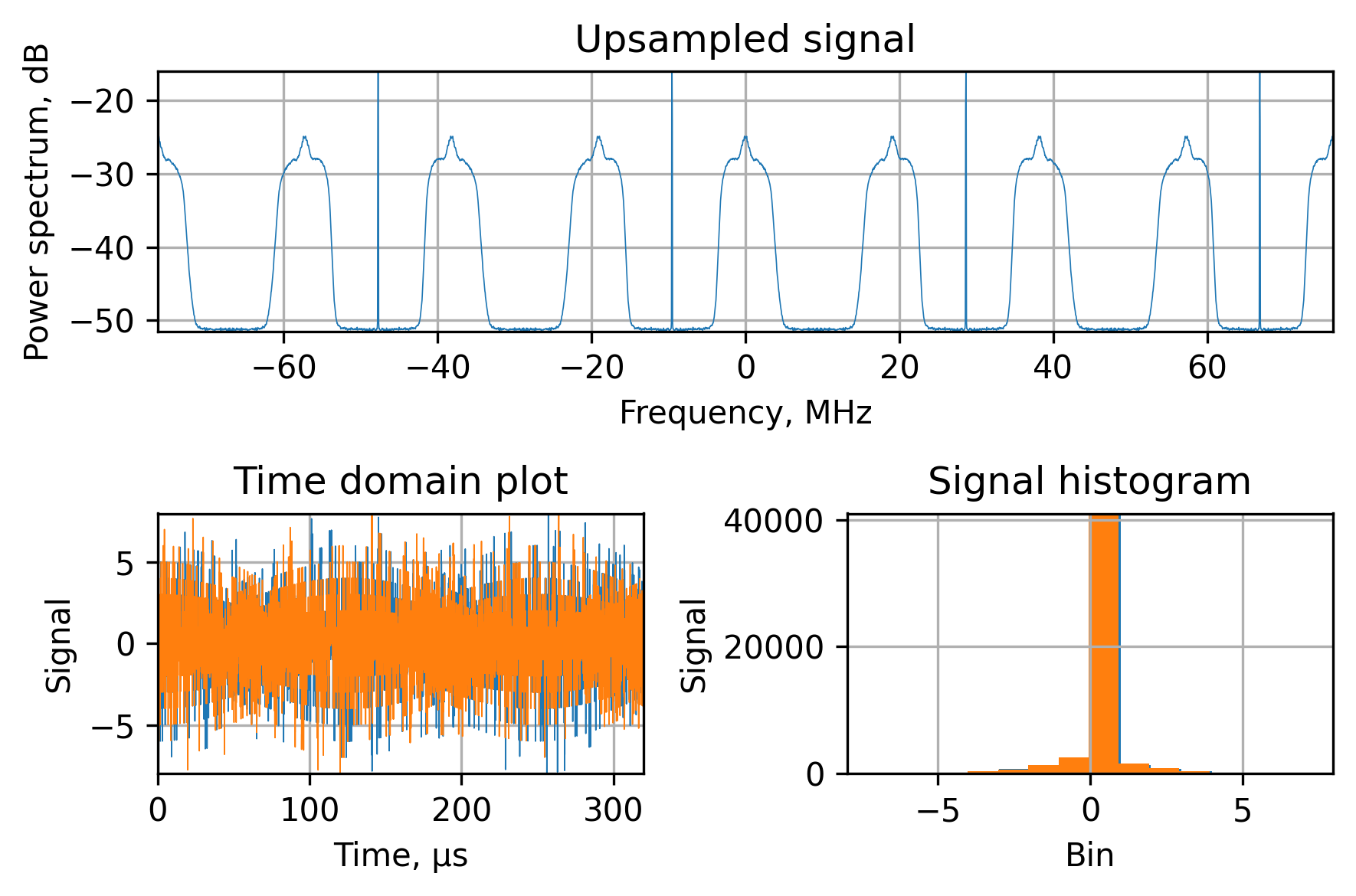
There are two main points in this signal:
- The spectrum is periodical and repeated. This is due to the properties of the digital signal
- The histogram shows a lot of zeros because for every normally distributed sample we’ve inserted $N - 1$ zeros.
Integer resampling is an expansion of the previous task with the downsampling follow-up. Downsampling may be viewed as an inverted upsampling: low-pass filtering with the following signal decimation (taking every $M$th sample). Downsampling filter types are the same with the only difference in cutoff frequency: $M\frac{f_{sOld}}{2}$.
Hardware-friendly optimizations
One of the hardware-efficient downsampling methods I’ve been using a lot in GNSS signal processing is accumulation, in which every output sample is the (normalized) sum of $M$ samples of the input samples.
For the sake of vectorization, interpreter-based languages can perform accumulation as a pair of reshaping and column-wise sums. Similar to the upsampling, the input vector \[\begin{pmatrix} s_0 \\ s_1 \\ \vdots \\ s_{M-1} \end{pmatrix}\]
is reshaped into the $(M / N, N)$ matrix \[\begin{pmatrix} s_0 & s_1 & \cdots & s_{N-1} \\ s_N & \vdots & \ddots & \vdots \\ \cdots & \cdots & \cdots & s_{M-1} \end{pmatrix}\]
and then being row-wise summed \[\begin{pmatrix} \sum_{i=0}^{N-1} s_i \\ \sum_{i=N}^{2N-1} s_i \\ \vdots \\ \end{pmatrix}\]
fs_down = fs / 4
time_down = np.arange(translated_signal.shape[0] / 4) / fs_down
reshaped = translated_signal.reshape((-1, 4))
accumulated = reshaped.sum(axis=1) / 4
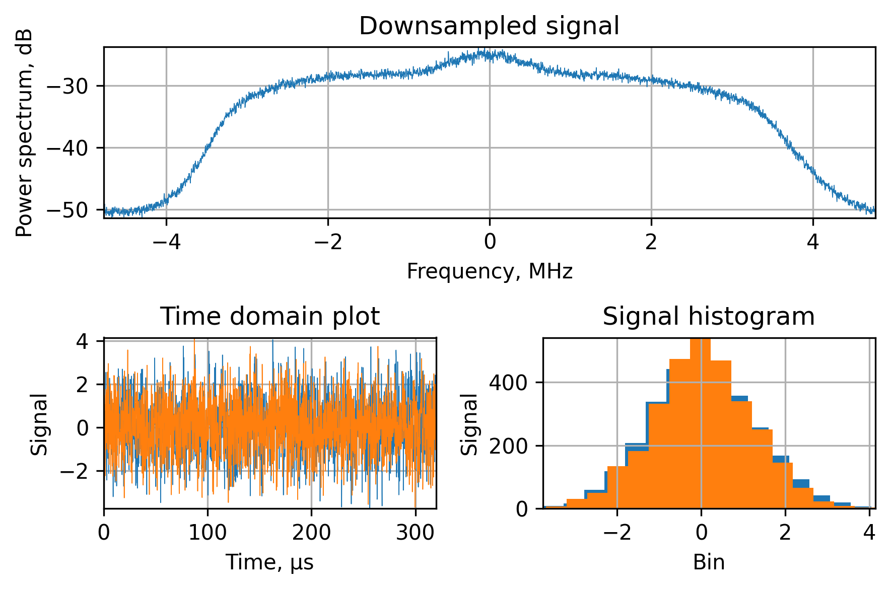
PlotSignal(accumulated, fs_down, 'Downsampled signal')
The point of accumulating is the implicit low-pass filtering with a $\frac{sin(x)}{x}$ frequency response, which is relatively inefficient from the high-frequency suppression point of view, but it’s one of the most easy-to-implement digital filters I’ve seen.
Signal packer
The final operation in the digital frontend is to save the final group signal into the local memory in the format, suitable for the used correlator implementation. This is a hardware-dependent block and all the possibilities should be thoroughly benchmarked.
One of the things worth pointing out here is that since the digital frontend can be treated as a continuation of the traditional analog RF frontend, it’s possible to interpret the signal packer as some kind of the ADC. For example, if there’s no interference present (or mitigated, more on that in Part 2: Jamming mitigation), the resulting signal can be stored with low precision: 1 or 2 bits, like the ADCs, used widely in GNSS frontends.
Another benefit of such low-precision signal storage is the possibility to implement the correlator block to operate on such packed data. It will allow to increase the throughput of the block and reduce the required silicon area.
Curiously, during my experiments with PC-based digital signal processing, the most performant versions turned out to be the float-based ones. This can be explained simply by the fact that with floats we’re only required to perform the operations we intend to: multiply, add, accumulate etc. On the other hand, if we’re dealing with integers (or even packed integers) the number of operations and memory accesses is increased because now it’s necessary to unpack the data, scale the result and pack it back.
Summary
This chapter has provided a brief overview and explanation of the digital frontend block for the software-defined GNSS receivers. It, by no means, is a necessary part of the receiver, but it provides enough flexibility for the system engineers to design the receiver tailored for the specific market and/or applications.
Using the digital frontend in the GNSS receiver design allows decoupling of the synchronous digital processing, performed at the ADC sampling rate, from the asynchronous correlation processing. This, in turn, helps to design a more flexible signal data flow with additional filtering and resampling.
Another essential part of the digital frontend is the jamming detection and mitigation block, but I’ve decided to dedicate a standalone chapter to it since the topic is very deep.