Global Navigation Satellite Systems Software-Defined Receivers explained. Part 3: Acquisition
Signal acquisition is a process of a rough estimation of partial code delay and pseudo-Doppler frequency to provide a bootstrap for the tracking loops. In the modern software-defined receivers there’s a designated hardware/software block called the Fast Search Engine (FSE) that is used to speed up the initialization of the receiver in the case of a cold start.
- Part 0: Hardware and system design
- Part 1: Digital frontend
- Part 2: Jamming mitigation
- Part 3: Acquisition
- Part 4: Correlation and tracking
- Part 5: Standalone positioning
- Part 6: Advanced positioning methods
Overview
Before we start with acquisition let’s revisit the model of the signal, simplified for one satellite in one frequency band without the multipath effect: \[s(t) = AC(t - \tau)D(t - \tau)e^{j2\pi (f + f_D) t + \phi_0} + n(t)\]
In that model $A$ represents the signal power, $\tau$ is the total code delay, $C(t - \tau)$ is the delayed ranging code, $D(t - \tau)$ is the delayed navigation data message, $f$ is the carrier frequency of the satellite, $f_D$ is the pseudo-Doppler frequency offset (more on the pseudo- part later), $\phi_0$ is the phase delay and the $n(t)$ is the additive noise of the receiver.
The goals of the acquisition engine are:
- Determine the partial code delay by estimating the ranging code $C(t - \tau)$ phase ($\tau\ \% {\ code\ duration}$)
- Evaluate the $f_D$ pseudo-Doppler frequency of the signal
- (Optional) Estimate the $D(t - \tau)$ navigation message partial phase (bit switch event)
A note about the pseudo- in the Doppler frequency offset
As you’re aware, the Doppler effect is the change of the signal frequency proportional to the radial velocity between the emitter and the observer. The radial velocity occurs when those two objects either approach or move away from each other.
I’m sorry for an offtopic, but this explanation is just hilarious:

The pure (so to speak) Doppler effect is observed when the observer is producing the initial signal as well with the same reference oscillator, for example, a traditional passive radar.
On the other hand, if the reference oscillators of the emitter and the observer aren’t the same, an additional frequency offset may be observed. To illustrate this, let’s imagine that a GPS satellite is in the zenith (directly above) and a (simplified) stationary receiver with a reference oscillator with a nominal frequency $f_{ref}$ of 10 MHz. However, due to the temperature and ageing, the frequency is slightly off, let’s say 9.99 MHz.
A simple single-conversion IQ RF frontend would use some kind of PLL to multiply the reference frequency $f_{ref}$ to become $f_{LO}$ of 1575.42 MHz. For the sake of simplicity, let’s assume a fractional-N PLL with a coefficient of 1575.42. If we multiply the “real” $f_{ref}$ with that coefficient we’ll get roughly 1573.84 MHz.
So simply because of the single heterodyne, we’ll get more than 1.57 MHz of an additional frequency shift, and we haven’t even started with the sampling effects of the ADC with the mismatched clock.
Thankfully, modern GNSS receivers use Temperature Compensated Crystal Oscillators (TCXO) as a standard option with good stability and accuracy for a reasonable price and the pseudo- part of the Doppler offset is kept within the tens and hundreds of Hz, but that’s something worth remembering.
It’s also worth pointing out that there are devices called GNSSDOs (GNSS-disciplined oscillators), that estimate the offset of the reference oscillator by an additional step in the positioning phase called the speed equation: by using the same maths on pseudo-Doppler shifts instead of the pseudoranges it’s possible to estimate the speed of the receiver and the clock drift (with $\frac{seconds}{seconds}$ dimension) instead of the coordinates and a clock shift with the traditional navigation equation.
The whole timing receivers and time scales is a deep and interesting topic, I highly recommend the Global synchronization and near-Earth movement control satellite systems (unfortunately, only in Russian) book by Prof. Povalyaev. It’s quite difficult to understand, but really worth it.
Fast Search Engine
As I’ve mentioned earlier, the acquisition engine is used to determine the partial delay and the pseudo-Doppler frequency offset. Therefore, the acquisition process may be treated as a 2-dimensional maximum search with a certain threshold. There are three customization points:
- Search range: usually, the whole code period for the delay axis and ±5 kHz for the pseudo-Doppler offset. The frequency range should be selected for the assumed receiver dynamics and the accuracy of the onboard reference oscillator
- Search step: determines the granularity and is defined by the initialization bandwidth of the (following) tracking loops on one hand and timing constraints on the other.
- Accumulation quantity and type: how many milliseconds we accumulate and how exactly the accumulation is performed (coherent vs non-coherent)
The acquisition process in GNSS receivers is operating in the so-called soft real-time mode.
A quick detour to explain the real-time operations and the difference between the modes:
The real-time is all about constraints and, technically speaking, isn’t about fast software. Depending on what are the effects of missing the processing deadline, three types of real-time modes can be highlighted:
- Non-real-time: this is the most widespread type of operation when no timeframe is specified.
- Soft real-time provides a timeframe for a response, but if the system misses the deadline user will observe a temporary degradation, following restoration. One of the great examples is a video player: if for some reason, the video frame is missed, the player will produce output with some artefacts, but the movie will continue to play.
- Hard real-time has a more strict timeframe, if you miss it the whole system is rendered useless. Therefore, hard real-time systems preferably run either bare-metal or with a thinnest scheduler-type pseudo-OS.
The software-friendly acquisition engine saves the signal samples synchronously upon receiving an acquisition request, followed by an asynchronous process of 2-dimensional search. The first step is to reduce the data rate to lower the number of required calculations. It is reasonable to reduce the sampling to the minimal feasible ($f_S= 2f_{code}$) due to the usage of the code tracking loops.
fs_acquisition = 2.046e6
samples_per_ms = int(fs_acquisition / 1e3)
ms_to_process = 4
acquisition_signal = signal.resample(translated_signal[0:int(ms_to_process * fs / 1e3)], int(ms_to_process * samples_per_ms))
The next step is to slice the 2-dimensional window of search into the consecutive iterations with fixed Doppler offset and run the matched filter calculations on the signal. The next step is the accumulation, finding the maximum (peak value and location) and comparing it with a threshold.
for doppler in range(-7000, 7000, 50):
  sine = np.exp(-1j * 2 * np.pi * doppler * time_acquisition)
  translated = (acquisition_signal * sine)
  matched_output = np.fft.ifft(np.fft.fft(translated) * np.conj(np.fft.fft(code)))
  matched_output_ms = matched_output.reshape((ms_to_process, samples_per_ms))
  if use_coherent_acquisition:
    matched_output_ms = np.abs(matched_output_ms.sum(axis=0))
  else:
    matched_output_ms = np.abs(matched_output_ms).sum(axis=0)

  current_peak_value = np.max(matched_output_ms)
  if current_peak_value > max_peak_value:
    max_peak_value = current_peak_value
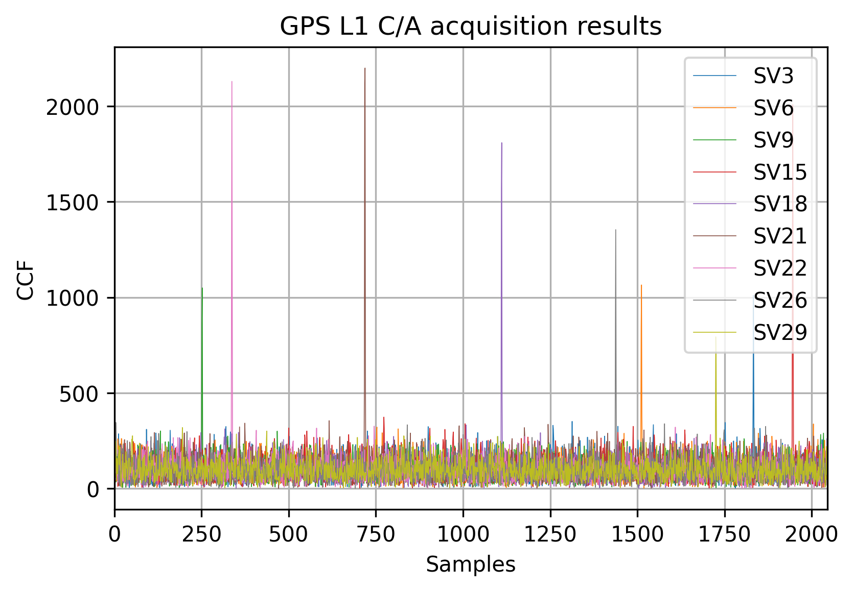
The result of the acquisition of all the GPS satellites can be illustrated like this:
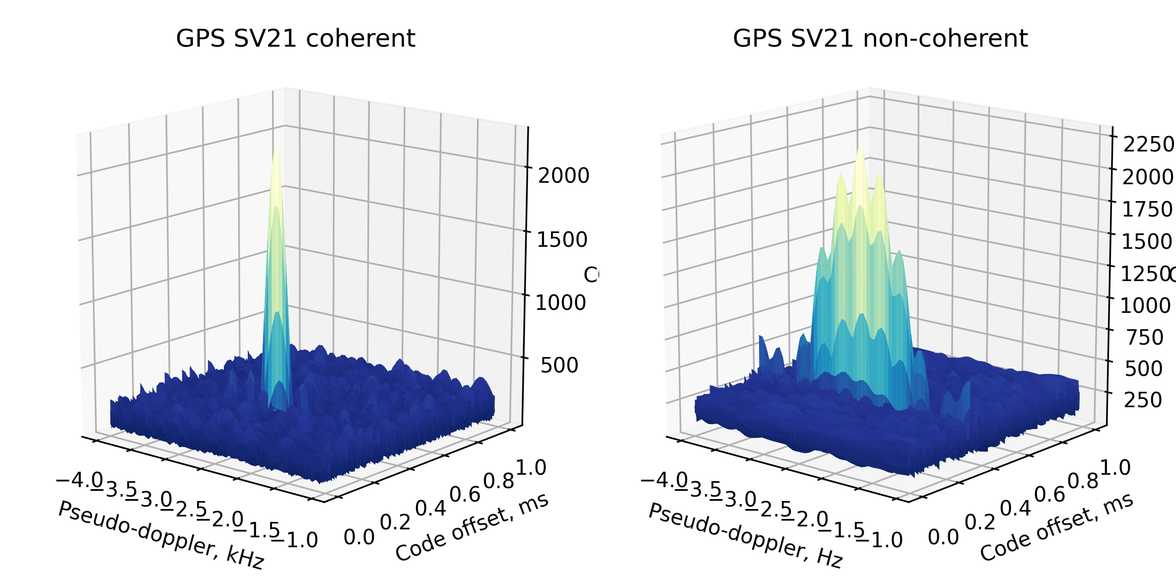
Accumulation in the acquisition
One of the important questions in the acquisition is accumulation. To increase the detection probability in case of the navigation message sign change or shadowing it’s common to operate on several consecutive milliseconds followed by accumulation. There are two approaches for accumulation: coherent and non-coherent.
In the acquisition routine we don’t care about the carrier phase the difference between the two types of accumulation is the order of the magnitude and sum operations:
matched_output_ms = matched_output.reshape((ms_to_process, samples_per_ms))
if use_coherent_acquisition:
  matched_output_ms = np.abs(matched_output_ms.sum(axis=0))
else:
  matched_output_ms = np.abs(matched_output_ms).sum(axis=0)
The coherent accumulation usually results in a more “sharp” 2-dimensional ambiguity body but has a major downside being prone to the navigational message sign bit change. For example, if working with 4 milliseconds and the first two are positive and the last two are negative, resulting in a massively decreased signal-to-noise ratio.
This is also the case for the relatively high-speed data transfer signals, like the SBAS L1 or the signals with overlay codes like the BeiDou B1I.
Matrix-oriented acquisition
The sliced approach, described above, is often used in memory-limited devices like ASICs or FPGAs. However, for PC-based receivers (both CPU- and GPU-based) a matrix-based algorithm can be used. It benefits from the pre-existing highly optimized matrix multiplication libraries and massively parallel architectures at the cost of higher memory consumption.
To illustrate this with an example we’ll use the following data:
- $N$ milliseconds of data at $f_S$ sampling rate, resulting in a $(\frac{N*f_S}{10^{-3}}, 1)$ vector, which we’ll denote as a $(n, 1)$ vector
- Vector of Doppler offset frequencies within the range of $\pm F_D$ Hz and a step of $\Delta f_D$ Hz, resulting in a $(1, \frac{2F_D + 1}{\Delta f_D})$ vector, which we’ll denote as a $(1, p)$ vector
To match the dimensions we’ll need to prepare a translation matrix of size $(n, p)$ by calculating the complex exponent of frequencies over the $N$ milliseconds (see the translation chapter).
To translate the input signal we’ll perform an elementwise multiplication of the input signal and the translation matrix, resulting in a matrix of the same size $(n, p)$.
The next step is to acquire the Fourier transform of those matrices, but keep in mind, that this would be the traditional 1-dimensional DFT and not the 2-dimensional DFT. This means that we need only the column-wise transform without the follow-up row-wise calculations. Ths upside here is that it can be paralleled to utilize the multicore architecture.
According to the convolution theorem, to get the result we’ll elementwise multiply the input matrix and the complex conjugated input code, followed by the inverse Fourier transform. Accumulation and maximum search is performed as in the usual acquisition engine, but with fewer temporary variables and better memory locality.
Fine acquisition and bit border detection
One of the nice little acquisition tricks up my sleeve I’ve learned during my university years is the combined fine acquisition and bit border detection. Usually, when there’s an acquisition candidate, the first tracking step is the frequency locked loop (FLL) for some time followed by a phase-locked loop (PLL). However, this approach may take some time to obtain stable tracking, up to several seconds.
The idea is that for each successful acquisition we run the correlator as-is, without any tracking attempts, for 32 milliseconds to see something like this:
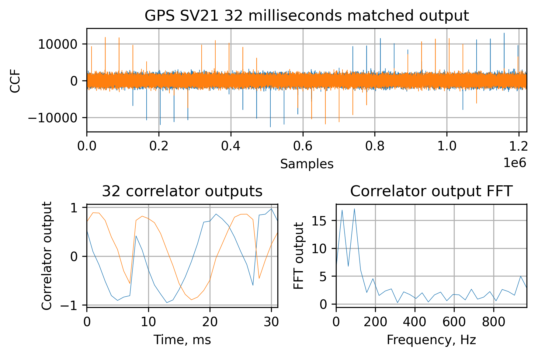
In the lower-left, you can see the correlator outputs and in the lower right the FFT output. As you can see, there are two low peaks in the spectrum of the correlator outputs. The fact that there are a finite number of bit shift combinations (I’ll leave it up to you to write them all down if you’d decide to implement this yourself) allows to test multiple hypotheses about the bit shift location and correct the Doppler frequency ambiguity to no more than a 32.5 Hz ($\frac{1000Hz}{32}$).
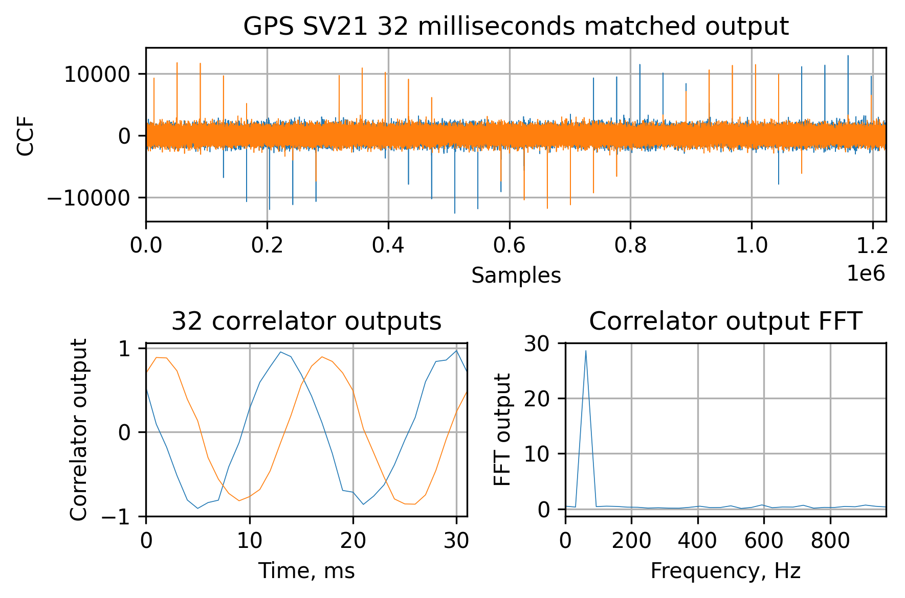
For example, with one of the combinations we can turn the sign-changing sine to the smooth one, fixing the 200 Hz Doppler offset and finding the sign change at the 8th millisecond:
Summary
Signal acquisition is an essential part of every GNSS receiver. The basic algorithm is the same, but the details are system- and signal-dependent. The traditional approach for multi-band receivers is to acquire whichever signal’s easier for you and use this data to bootstrap the tracking in the other frequency bands.
The main challenge in the acquisition algorithms, in my opinion, is overcoming the memory and computational limits and implementing everything accurately because acquisition sensitivity is usually much lower than the tracking, therefore errors and mismatches here and there may lead to even further degradation.